【OptunaでSHAP】ハイパーパラメータ探索での寄与率を計算してみた
optunaのv3のベータ版(v3.0.0b1)が公開された。リリース情報を見ていて個人的に気になったのがSHAP値の計算機能の追加であった。
SHAPは調べるといろいろな人が「使ってみた」や解説記事を書いているので詳細な説明はそれに譲るが、簡単に言えばどの特徴量やパラメータが予測に対してどのくらい寄与しているかを評価することができる。
これをoptunaに実装し、ハイパーパラメータチューニングの最中にどれくらいどのパラメータが影響を与えたかを簡単に確認することができる機能が実装されたので使ってみる。
環境
M1のMacbook Air (2020)
sw_vers
ProductName:    macOS
ProductVersion: 12.4
BuildVersion:   21F79
python環境はm1ネイティブのminiforgeを使用し、仮想環境を構築した。
conda create -n optuna-shap python=3.9 --file requirements-conda.txt
なお、requirements-conda.txtの内容は以下。
tqdm
SQLAlchemy>=1.1.0
typing-extensions
PyYAML
cliff
colorlog
cmaes>=0.8.2
alembic
Mako
pbr!=2.1.0,>=2.0.0
PrettyTable>=0.7.2
stevedore>=2.0.1
autopage>=0.4.0
cmd2>=1.0.0
pyperclip>=1.6
jupyter
scikit-learn
matplotlib
pandas
plotly
shap
いろいろなパッケージを書いたが、optunaのベータ版をpipからインストールすることに起因する。pipからインストールせざるを得ないが、できる限りpipとcondaを混在させたくないために、optuna以外をconda installするために指定した結果である。このあと以下のコマンドで仮想環境をactivateし、pipでベータ版のoptuna (v3.0.0b1)をダウンロードした。
conda activate optuna-shap
pip install optuna==3.0.0b1
コード
モジュールのインポート
from sklearn.ensemble import RandomForestRegressor
from sklearn.model_selection import cross_validate, KFold
from sklearn.base import clone
import optuna
from optuna.integration.shap import ShapleyImportanceEvaluator
import matplotlib.pyplot as plt
import matplotlib as mpl
import seaborn as sns
from urllib import request
import os
import pandas as pd
サンプルデータのダウンロード
金子研究室にて配布されている有機化合物の溶解度予測用データセット(回帰)を利用。本来は有機化合物の構造から特徴量を作成するためにはrdkitが必要であるが、すでに特徴量が作成されてcsvにされたものが配布されているのでこちらを利用する。
以下ではサーバーに負荷をかけてご迷惑をかけないために一度ダウンロードしたらそのキャッシュを使用するようにした。
# 配布ページ: https://datachemeng.com/pythonassignment/
url = 'https://datachemeng.com/wp-content/uploads/2017/07/logSdataset1290.csv'

dirpath_cache = os.path.abspath('./_cache')
if not os.path.isdir(dirpath_cache):
    os.mkdir(dirpath_cache)

fpath_csv_cache = os.path.join(dirpath_cache, os.path.basename(url))
if not os.path.isfile(fpath_csv_cache):
    with request.urlopen(url) as response:
        content = response.read().decode('utf-8-sig')
    with open(fpath_csv_cache, 'w', encoding='utf-8-sig') as f:
        f.write(content)

df_data = pd.read_csv(fpath_csv_cache, index_col=0)
df_data.head()
| logS | MolWt | HeavyAtomMolWt | ExactMolWt | NumValenceElectrons | NumRadicalElectrons | MaxPartialCharge | MinPartialCharge | MaxAbsPartialCharge | MinAbsPartialCharge | ... | fr_sulfide | fr_sulfonamd | fr_sulfone | fr_term_acetylene | fr_tetrazole | fr_thiazole | fr_thiocyan | fr_thiophene | fr_unbrch_alkane | fr_urea | |
|---|---|---|---|---|---|---|---|---|---|---|---|---|---|---|---|---|---|---|---|---|---|
| CC(N)=O | 1.58 | 59.068 | 54.028 | 59.037114 | 24 | 0 | 0.213790 | -0.369921 | 0.369921 | 0.213790 | ... | 0 | 0 | 0 | 0 | 0 | 0 | 0 | 0 | 0 | 0 |
| CNN | 1.34 | 46.073 | 40.025 | 46.053098 | 20 | 0 | -0.001725 | -0.271722 | 0.271722 | 0.001725 | ... | 0 | 0 | 0 | 0 | 0 | 0 | 0 | 0 | 0 | 0 |
| CC(=O)O | 1.22 | 60.052 | 56.020 | 60.021129 | 24 | 0 | 0.299685 | -0.481433 | 0.481433 | 0.299685 | ... | 0 | 0 | 0 | 0 | 0 | 0 | 0 | 0 | 0 | 0 |
| C1CCNC1 | 1.15 | 71.123 | 62.051 | 71.073499 | 30 | 0 | -0.004845 | -0.316731 | 0.316731 | 0.004845 | ... | 0 | 0 | 0 | 0 | 0 | 0 | 0 | 0 | 0 | 0 |
| NC(=O)NO | 1.12 | 76.055 | 72.023 | 76.027277 | 30 | 0 | 0.335391 | -0.349891 | 0.349891 | 0.335391 | ... | 0 | 0 | 0 | 0 | 0 | 0 | 0 | 0 | 0 | 1 |
5 rows × 197 columns
再現性のためのシード値の固定。
SEED = 334
説明変数と目的変数に分離。
col_target = 'logS'
X = df_data.drop(col_target, axis=1)
y = df_data[col_target]
X.head()
| MolWt | HeavyAtomMolWt | ExactMolWt | NumValenceElectrons | NumRadicalElectrons | MaxPartialCharge | MinPartialCharge | MaxAbsPartialCharge | MinAbsPartialCharge | MaxEStateIndex | ... | fr_sulfide | fr_sulfonamd | fr_sulfone | fr_term_acetylene | fr_tetrazole | fr_thiazole | fr_thiocyan | fr_thiophene | fr_unbrch_alkane | fr_urea | |
|---|---|---|---|---|---|---|---|---|---|---|---|---|---|---|---|---|---|---|---|---|---|
| CC(N)=O | 59.068 | 54.028 | 59.037114 | 24 | 0 | 0.213790 | -0.369921 | 0.369921 | 0.213790 | 9.222222 | ... | 0 | 0 | 0 | 0 | 0 | 0 | 0 | 0 | 0 | 0 |
| CNN | 46.073 | 40.025 | 46.053098 | 20 | 0 | -0.001725 | -0.271722 | 0.271722 | 0.001725 | 4.597222 | ... | 0 | 0 | 0 | 0 | 0 | 0 | 0 | 0 | 0 | 0 |
| CC(=O)O | 60.052 | 56.020 | 60.021129 | 24 | 0 | 0.299685 | -0.481433 | 0.481433 | 0.299685 | 9.000000 | ... | 0 | 0 | 0 | 0 | 0 | 0 | 0 | 0 | 0 | 0 |
| C1CCNC1 | 71.123 | 62.051 | 71.073499 | 30 | 0 | -0.004845 | -0.316731 | 0.316731 | 0.004845 | 3.222222 | ... | 0 | 0 | 0 | 0 | 0 | 0 | 0 | 0 | 0 | 0 |
| NC(=O)NO | 76.055 | 72.023 | 76.027277 | 30 | 0 | 0.335391 | -0.349891 | 0.349891 | 0.335391 | 9.229167 | ... | 0 | 0 | 0 | 0 | 0 | 0 | 0 | 0 | 0 | 1 |
5 rows × 196 columns
ハイパーパラメータ探索への準備
今回は簡単のため、ランダムフォレストを使用。
rf = RandomForestRegressor(random_state=SEED, n_jobs=-1)
ハイパーパラメータ探索用の目的関数の定義
def objective(trial:optuna.trial.Trial) -> float:
    params = {
        'n_estimators': trial.suggest_int('n_estimators', 1, 100),
        'max_depth': trial.suggest_int('max_depth', 1, 10),
        'min_samples_split': trial.suggest_uniform('min_samples_split', 0.1, 1.0),
        'min_samples_leaf': trial.suggest_uniform('min_samples_leaf', 0.1, 1.0),
    }
    kf = KFold(n_splits=5, shuffle=True, random_state=SEED)
    cv_score = cross_validate(clone(rf).set_params(**params), X, y, cv=kf, scoring='neg_mean_squared_error', return_train_score=False, n_jobs=-1)
    return -cv_score['test_score'].mean()
テスト用のトライアルケースを準備
trial_test = optuna.trial.FixedTrial({
    'n_estimators': 100,
    'max_depth': 5,
    'min_samples_split': 2,
    'min_samples_leaf': 1
})
テストを実施
objective(trial_test)
suggest_uniform has been deprecated in v3.0.0. This feature will be removed in v6.0.0. See https://github.com/optuna/optuna/releases/tag/v3.0.0. Use :func:`~optuna.trial.FixedTrial.suggest_float` instead.
The value 2 of the parameter 'min_samples_split' is out of the range of the distribution FloatDistribution(high=1.0, log=False, low=0.1, step=None).
suggest_uniform has been deprecated in v3.0.0. This feature will be removed in v6.0.0. See https://github.com/optuna/optuna/releases/tag/v3.0.0. Use :func:`~optuna.trial.FixedTrial.suggest_float` instead.


0.4311507013000121
suggest_uniformはdeprecatedになるらしい。知らなかった。suggest_floatに移行していく感じらしい。
ハイパーパラメータ探索
sampler = optuna.samplers.TPESampler(seed=SEED)
study = optuna.create_study(sampler=sampler, direction='maximize')
study.optimize(objective, n_trials=50)
[32m[I 2022-06-11 17:31:49,556][0m A new study created in memory with name: no-name-8ae21fd3-ed79-473d-b95f-81af69a35113[0m
suggest_uniform has been deprecated in v3.0.0. This feature will be removed in v6.0.0. See https://github.com/optuna/optuna/releases/tag/v3.0.0. Use :func:`~optuna.trial.Trial.suggest_float` instead.
suggest_uniform has been deprecated in v3.0.0. This feature will be removed in v6.0.0. See https://github.com/optuna/optuna/releases/tag/v3.0.0. Use :func:`~optuna.trial.Trial.suggest_float` instead.
[32m[I 2022-06-11 17:31:50,207][0m Trial 0 finished with value: 1.9372632750738048 and parameters: {'n_estimators': 24, 'max_depth': 1, 'min_samples_split': 0.21184083616914012, 'min_samples_leaf': 0.25349329561749007}. Best is trial 0 with value: 1.9372632750738048.[0m
[32m[I 2022-06-11 17:31:50,695][0m Trial 1 finished with value: 4.131692722779455 and parameters: {'n_estimators': 30, 'max_depth': 9, 'min_samples_split': 0.8194036224693542, 'min_samples_leaf': 0.19587780028459273}. Best is trial 1 with value: 4.131692722779455.[0m
[32m[I 2022-06-11 17:31:50,916][0m Trial 2 finished with value: 4.1320406119102415 and parameters: {'n_estimators': 84, 'max_depth': 6, 'min_samples_split': 0.8406086066912434, 'min_samples_leaf': 0.648148242466285}. Best is trial 2 with value: 4.1320406119102415.[0m
[32m[I 2022-06-11 17:31:51,276][0m Trial 3 finished with value: 1.7955958804257022 and parameters: {'n_estimators': 77, 'max_depth': 1, 'min_samples_split': 0.5703368992433854, 'min_samples_leaf': 0.1697862849949252}. Best is trial 2 with value: 4.1320406119102415.[0m
[32m[I 2022-06-11 17:31:51,478][0m Trial 4 finished with value: 4.131988507396857 and parameters: {'n_estimators': 53, 'max_depth': 8, 'min_samples_split': 0.647745177089535, 'min_samples_leaf': 0.5735971070115229}. Best is trial 2 with value: 4.1320406119102415.[0m
[32m[I 2022-06-11 17:31:51,870][0m Trial 5 finished with value: 1.7334918121364826 and parameters: {'n_estimators': 96, 'max_depth': 4, 'min_samples_split': 0.6100316949260556, 'min_samples_leaf': 0.12863019715689822}. Best is trial 2 with value: 4.1320406119102415.[0m
[32m[I 2022-06-11 17:31:52,110][0m Trial 6 finished with value: 4.131968898539031 and parameters: {'n_estimators': 54, 'max_depth': 1, 'min_samples_split': 0.36709906006096704, 'min_samples_leaf': 0.6774946467008782}. Best is trial 2 with value: 4.1320406119102415.[0m
[32m[I 2022-06-11 17:31:52,292][0m Trial 7 finished with value: 4.131698083892635 and parameters: {'n_estimators': 22, 'max_depth': 5, 'min_samples_split': 0.9360920363852169, 'min_samples_leaf': 0.5314363048393248}. Best is trial 2 with value: 4.1320406119102415.[0m
[32m[I 2022-06-11 17:31:52,522][0m Trial 8 finished with value: 4.132000012250806 and parameters: {'n_estimators': 96, 'max_depth': 5, 'min_samples_split': 0.7889147214024875, 'min_samples_leaf': 0.17587131137545817}. Best is trial 2 with value: 4.1320406119102415.[0m
[32m[I 2022-06-11 17:31:52,724][0m Trial 9 finished with value: 4.131709376057453 and parameters: {'n_estimators': 21, 'max_depth': 3, 'min_samples_split': 0.2344239741915438, 'min_samples_leaf': 0.944909589532148}. Best is trial 2 with value: 4.1320406119102415.[0m
[32m[I 2022-06-11 17:31:52,935][0m Trial 10 finished with value: 4.132127543029714 and parameters: {'n_estimators': 73, 'max_depth': 7, 'min_samples_split': 0.9998177612110161, 'min_samples_leaf': 0.8647884881265333}. Best is trial 10 with value: 4.132127543029714.[0m
[32m[I 2022-06-11 17:31:53,172][0m Trial 11 finished with value: 4.132127543029714 and parameters: {'n_estimators': 73, 'max_depth': 7, 'min_samples_split': 0.9746725999595544, 'min_samples_leaf': 0.8674795576878556}. Best is trial 10 with value: 4.132127543029714.[0m
[32m[I 2022-06-11 17:31:53,389][0m Trial 12 finished with value: 4.132074030323225 and parameters: {'n_estimators': 71, 'max_depth': 7, 'min_samples_split': 0.975648016015977, 'min_samples_leaf': 0.9957835502494556}. Best is trial 10 with value: 4.132127543029714.[0m
[32m[I 2022-06-11 17:31:53,598][0m Trial 13 finished with value: 4.132073044897243 and parameters: {'n_estimators': 68, 'max_depth': 10, 'min_samples_split': 0.730049961836955, 'min_samples_leaf': 0.7944194568441575}. Best is trial 10 with value: 4.132127543029714.[0m
[32m[I 2022-06-11 17:31:53,704][0m Trial 14 finished with value: 4.131888706024215 and parameters: {'n_estimators': 39, 'max_depth': 7, 'min_samples_split': 0.4539571681646011, 'min_samples_leaf': 0.8120251436456043}. Best is trial 10 with value: 4.132127543029714.[0m
[32m[I 2022-06-11 17:31:53,928][0m Trial 15 finished with value: 4.132047734070271 and parameters: {'n_estimators': 60, 'max_depth': 8, 'min_samples_split': 0.9041559728086773, 'min_samples_leaf': 0.40458987699210397}. Best is trial 10 with value: 4.132127543029714.[0m
[32m[I 2022-06-11 17:31:54,084][0m Trial 16 finished with value: 4.132008509883346 and parameters: {'n_estimators': 2, 'max_depth': 10, 'min_samples_split': 0.9841078499880017, 'min_samples_leaf': 0.8540978674766526}. Best is trial 10 with value: 4.132127543029714.[0m
[32m[I 2022-06-11 17:31:54,308][0m Trial 17 finished with value: 4.132055216344758 and parameters: {'n_estimators': 85, 'max_depth': 7, 'min_samples_split': 0.6782569408181941, 'min_samples_leaf': 0.7417538815569331}. Best is trial 10 with value: 4.132127543029714.[0m
[32m[I 2022-06-11 17:31:54,521][0m Trial 18 finished with value: 4.1320384183342656 and parameters: {'n_estimators': 64, 'max_depth': 6, 'min_samples_split': 0.4416712017486114, 'min_samples_leaf': 0.9038472667488379}. Best is trial 10 with value: 4.132127543029714.[0m
[32m[I 2022-06-11 17:31:54,724][0m Trial 19 finished with value: 4.131947050579607 and parameters: {'n_estimators': 42, 'max_depth': 3, 'min_samples_split': 0.8529877521765832, 'min_samples_leaf': 0.4400722555619374}. Best is trial 10 with value: 4.132127543029714.[0m
[32m[I 2022-06-11 17:31:54,933][0m Trial 20 finished with value: 4.1320406119102415 and parameters: {'n_estimators': 84, 'max_depth': 8, 'min_samples_split': 0.7254146327572326, 'min_samples_leaf': 0.7121650222636289}. Best is trial 10 with value: 4.132127543029714.[0m
[32m[I 2022-06-11 17:31:55,139][0m Trial 21 finished with value: 4.132086887086807 and parameters: {'n_estimators': 72, 'max_depth': 7, 'min_samples_split': 0.9663212033087448, 'min_samples_leaf': 0.997351740648774}. Best is trial 10 with value: 4.132127543029714.[0m
[32m[I 2022-06-11 17:31:55,347][0m Trial 22 finished with value: 4.132011345203823 and parameters: {'n_estimators': 76, 'max_depth': 9, 'min_samples_split': 0.997205413227887, 'min_samples_leaf': 0.9873623652124208}. Best is trial 10 with value: 4.132127543029714.[0m
[32m[I 2022-06-11 17:31:55,557][0m Trial 23 finished with value: 4.132029209933387 and parameters: {'n_estimators': 58, 'max_depth': 6, 'min_samples_split': 0.9010749455713001, 'min_samples_leaf': 0.8890315024089664}. Best is trial 10 with value: 4.132127543029714.[0m
[32m[I 2022-06-11 17:31:55,744][0m Trial 24 finished with value: 4.1320725072374325 and parameters: {'n_estimators': 45, 'max_depth': 7, 'min_samples_split': 0.891806901438772, 'min_samples_leaf': 0.8052318780100712}. Best is trial 10 with value: 4.132127543029714.[0m
[32m[I 2022-06-11 17:31:55,947][0m Trial 25 finished with value: 4.132050035213429 and parameters: {'n_estimators': 75, 'max_depth': 9, 'min_samples_split': 0.7741976631796516, 'min_samples_leaf': 0.9334342928109846}. Best is trial 10 with value: 4.132127543029714.[0m
[32m[I 2022-06-11 17:31:56,174][0m Trial 26 finished with value: 4.132055216344758 and parameters: {'n_estimators': 85, 'max_depth': 5, 'min_samples_split': 0.996632074648519, 'min_samples_leaf': 0.8387676276943021}. Best is trial 10 with value: 4.132127543029714.[0m
[32m[I 2022-06-11 17:31:56,395][0m Trial 27 finished with value: 4.132022997337787 and parameters: {'n_estimators': 91, 'max_depth': 8, 'min_samples_split': 0.14059135913568083, 'min_samples_leaf': 0.7557316656995946}. Best is trial 10 with value: 4.132127543029714.[0m
[32m[I 2022-06-11 17:31:56,605][0m Trial 28 finished with value: 4.132013498142127 and parameters: {'n_estimators': 63, 'max_depth': 4, 'min_samples_split': 0.9196410265301609, 'min_samples_leaf': 0.6002638095723944}. Best is trial 10 with value: 4.132127543029714.[0m
[32m[I 2022-06-11 17:31:56,856][0m Trial 29 finished with value: 4.132086887086807 and parameters: {'n_estimators': 72, 'max_depth': 6, 'min_samples_split': 0.8603318711871742, 'min_samples_leaf': 0.48738808589239785}. Best is trial 10 with value: 4.132127543029714.[0m
[32m[I 2022-06-11 17:31:57,073][0m Trial 30 finished with value: 4.132052444928407 and parameters: {'n_estimators': 67, 'max_depth': 7, 'min_samples_split': 0.7567984733828065, 'min_samples_leaf': 0.3024301443890308}. Best is trial 10 with value: 4.132127543029714.[0m
[32m[I 2022-06-11 17:31:57,286][0m Trial 31 finished with value: 4.132011345203823 and parameters: {'n_estimators': 76, 'max_depth': 6, 'min_samples_split': 0.8624875923861973, 'min_samples_leaf': 0.4868893294231152}. Best is trial 10 with value: 4.132127543029714.[0m
[32m[I 2022-06-11 17:31:57,508][0m Trial 32 finished with value: 4.132069230669385 and parameters: {'n_estimators': 80, 'max_depth': 6, 'min_samples_split': 0.9410271214162161, 'min_samples_leaf': 0.3601711346530612}. Best is trial 10 with value: 4.132127543029714.[0m
[32m[I 2022-06-11 17:31:57,731][0m Trial 33 finished with value: 4.132061965987992 and parameters: {'n_estimators': 90, 'max_depth': 9, 'min_samples_split': 0.8206109767219647, 'min_samples_leaf': 0.6479239945619912}. Best is trial 10 with value: 4.132127543029714.[0m
[32m[I 2022-06-11 17:31:57,934][0m Trial 34 finished with value: 4.132086887086807 and parameters: {'n_estimators': 72, 'max_depth': 7, 'min_samples_split': 0.9378793184722503, 'min_samples_leaf': 0.8719609131915469}. Best is trial 10 with value: 4.132127543029714.[0m
[32m[I 2022-06-11 17:31:58,131][0m Trial 35 finished with value: 4.13203797756323 and parameters: {'n_estimators': 49, 'max_depth': 8, 'min_samples_split': 0.8457603022697052, 'min_samples_leaf': 0.5020339597326252}. Best is trial 10 with value: 4.132127543029714.[0m
[32m[I 2022-06-11 17:31:58,345][0m Trial 36 finished with value: 4.132015055025223 and parameters: {'n_estimators': 57, 'max_depth': 6, 'min_samples_split': 0.8078971597291934, 'min_samples_leaf': 0.6204535510275817}. Best is trial 10 with value: 4.132127543029714.[0m
[32m[I 2022-06-11 17:31:58,560][0m Trial 37 finished with value: 4.132069230669385 and parameters: {'n_estimators': 80, 'max_depth': 4, 'min_samples_split': 0.6867421408164478, 'min_samples_leaf': 0.8795851739708105}. Best is trial 10 with value: 4.132127543029714.[0m
[32m[I 2022-06-11 17:31:58,743][0m Trial 38 finished with value: 4.131828481336025 and parameters: {'n_estimators': 34, 'max_depth': 7, 'min_samples_split': 0.9470899396735694, 'min_samples_leaf': 0.9718148474983636}. Best is trial 10 with value: 4.132127543029714.[0m
[32m[I 2022-06-11 17:31:58,975][0m Trial 39 finished with value: 4.132046175007793 and parameters: {'n_estimators': 100, 'max_depth': 5, 'min_samples_split': 0.54342220236808, 'min_samples_leaf': 0.5627687984605746}. Best is trial 10 with value: 4.132127543029714.[0m
[32m[I 2022-06-11 17:31:59,189][0m Trial 40 finished with value: 4.132061965987992 and parameters: {'n_estimators': 90, 'max_depth': 8, 'min_samples_split': 0.9497045460953419, 'min_samples_leaf': 0.9140519603738936}. Best is trial 10 with value: 4.132127543029714.[0m
[32m[I 2022-06-11 17:31:59,423][0m Trial 41 finished with value: 4.132086887086807 and parameters: {'n_estimators': 72, 'max_depth': 7, 'min_samples_split': 0.8594712406307473, 'min_samples_leaf': 0.9467333158866243}. Best is trial 10 with value: 4.132127543029714.[0m
[32m[I 2022-06-11 17:31:59,631][0m Trial 42 finished with value: 4.132053687644824 and parameters: {'n_estimators': 70, 'max_depth': 7, 'min_samples_split': 0.8959136886194192, 'min_samples_leaf': 0.9462023475905197}. Best is trial 10 with value: 4.132127543029714.[0m
[32m[I 2022-06-11 17:31:59,837][0m Trial 43 finished with value: 4.132013498142127 and parameters: {'n_estimators': 63, 'max_depth': 6, 'min_samples_split': 0.9651975558103875, 'min_samples_leaf': 0.8475336519121451}. Best is trial 10 with value: 4.132127543029714.[0m
[32m[I 2022-06-11 17:32:00,062][0m Trial 44 finished with value: 4.132069230669385 and parameters: {'n_estimators': 80, 'max_depth': 5, 'min_samples_split': 0.8620436292843531, 'min_samples_leaf': 0.9955437480300418}. Best is trial 10 with value: 4.132127543029714.[0m
[32m[I 2022-06-11 17:32:00,305][0m Trial 45 finished with value: 4.132127543029714 and parameters: {'n_estimators': 73, 'max_depth': 9, 'min_samples_split': 0.5840653109143183, 'min_samples_leaf': 0.770531868234081}. Best is trial 10 with value: 4.132127543029714.[0m
[32m[I 2022-06-11 17:32:00,501][0m Trial 46 finished with value: 4.131967888054467 and parameters: {'n_estimators': 51, 'max_depth': 10, 'min_samples_split': 0.25892980239176655, 'min_samples_leaf': 0.7589548951442415}. Best is trial 10 with value: 4.132127543029714.[0m
[32m[I 2022-06-11 17:32:00,706][0m Trial 47 finished with value: 4.132052444928407 and parameters: {'n_estimators': 67, 'max_depth': 8, 'min_samples_split': 0.5929537786124391, 'min_samples_leaf': 0.6931892343754806}. Best is trial 10 with value: 4.132127543029714.[0m
[32m[I 2022-06-11 17:32:00,901][0m Trial 48 finished with value: 4.1319600422749305 and parameters: {'n_estimators': 55, 'max_depth': 9, 'min_samples_split': 0.36765774398132234, 'min_samples_leaf': 0.7882505125737362}. Best is trial 10 with value: 4.132127543029714.[0m
[32m[I 2022-06-11 17:32:01,241][0m Trial 49 finished with value: 1.9521491207403052 and parameters: {'n_estimators': 80, 'max_depth': 8, 'min_samples_split': 0.5010231706918343, 'min_samples_leaf': 0.2598001469501341}. Best is trial 10 with value: 4.132127543029714.[0m
SHAP値の確認
めちゃくちゃ簡単で、studyオブジェクトとSHAP値計算用のインスタンスを渡してあげれば良い。すると、plotlyを使って良い感じのグラフを作ってくれる。plotlyがないと以下のグラフ描画はエラーになるが、optuna自体のrequirementには現時点で入っていない。したがって、自分でダウンロードする必要がある。
optuna.visualization.plot_param_importances(study, evaluator=ShapleyImportanceEvaluator(seed=SEED))
ShapleyImportanceEvaluator is experimental (supported from v3.0.0). The interface can change in the future.
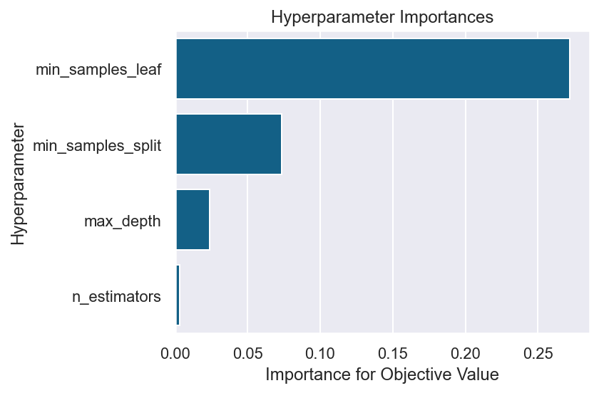
ちなみにmatplotlibでもできる。
optuna.visualization.matplotlib.plot_param_importances(study, evaluator=ShapleyImportanceEvaluator(seed=SEED))
/var/folders/81/n__nnfgd0zbf9m67d0jvmx_c0000gn/T/ipykernel_2553/425946331.py:1: ExperimentalWarning:

ShapleyImportanceEvaluator is experimental (supported from v3.0.0). The interface can change in the future.

/var/folders/81/n__nnfgd0zbf9m67d0jvmx_c0000gn/T/ipykernel_2553/425946331.py:1: ExperimentalWarning:

plot_param_importances is experimental (supported from v2.2.0). The interface can change in the future.


<AxesSubplot:title={'center':'Hyperparameter Importances'}, xlabel='Importance for Objective Value', ylabel='Hyperparameter'>
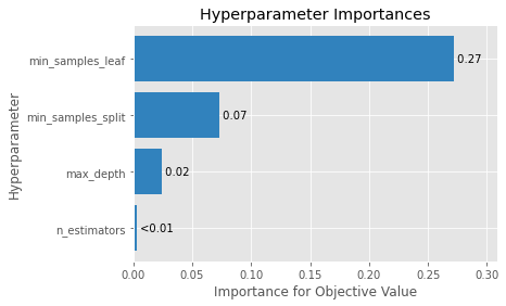
これだけで描画できる。素晴らしい。
今回MSEを評価項目としたので、min_sample_leafがMSEに対して0.27程度の影響を与えていることがわかる。
なお、seedを指定しないと結果が微妙にズレるので指定することをオススメする。
もう少し詳しく
これだとカスタマイズがあまり効かないので、自力で同じようなグラフを作ってみる。
ShapleyImportanceEvaluatorの公式ドキュメントを見てみるとevaluateモジュールを使えば計算できそうなので計算してみる。
# ignore optuna's experimental warnings
warnings.filterwarnings('ignore', category=optuna.exceptions.ExperimentalWarning)

evaluator = ShapleyImportanceEvaluator(seed=SEED)
importances = evaluator.evaluate(study)
importances
OrderedDict([('min_samples_leaf', 0.27189964137458184),
             ('min_samples_split', 0.07344403282773004),
             ('max_depth', 0.024016461643093377),
             ('n_estimators', 0.003185782057350999)])
collections.OrderDictオブジェクトが返ってくる。おそらく、寄与率の高い順番に結果を出力したいが、Python3.6まで辞書が順番を保存しなかったので、それをサポートしているためにOrderDictを使用しているのだと思う。
seabornでグラフ化
棒グラフの先に値が書いてはいないが、大体再現するとこんな感じ。これを基準にimportanceの値を加えるもよし、色を変えるもよしで色々カスタマイズができそう。
fig = plt.figure(dpi=144, facecolor='w')
sns.set_theme(style="darkgrid")
sns.barplot(data=pd.DataFrame.from_dict(importances, orient='index').transpose(), orient='h', color='#006699')
ax:plt.Axes = plt.gca()
ax.set_xlabel('Importance for Objective Value')
ax.set_ylabel('Hyperparameter')
ax.set_title('Hyperparameter Importances')
fig.tight_layout()
良い感じ。
まとめ
ハイパーパラメータ探索におけるSHAP値を簡単に算出・可視化できる。
コメント
この結果をもとに、ハイパーパラメータの探索要否を検討し、次回のモデル更新時は時間削減のためにこのパラメータは探索しない、などと利用ができそうだなと思った。
また、これによりなんとなくこの範囲でパラメータの探索をしよう、みたいなことが減りそう。
正式リリースが待たれる。