フィンガープリントによる部分構造の可視化について
マテリアルズインフォマティクス (MI) において最も重要な要素のうちの一つとして、モデルの解釈が挙げられる。
モデルを解釈することで、ドメイン知識と照らし合わせてモデルの正しさを確認することや新たな知見を得ることができる。
化学構造とその化合物の性質を紐づけて解析を行う定量的構造物性相関 (Quantitative Structure-Property Relationship, QSPR) 手法のうちの一つとして、FingerPrintを説明変数、化合物の性質を目的変数として機械学習モデルを構築する方法がある。
この手法について調査したところ、FingerPrintが対応する部分構造とそれに紐づく寄与率を化学構造上に描画することで解釈を行う手法があることがわかった。
これについて検討を行い、実際に描画を行なった結果を以下に示す。
概要
論文中では、溶解度予測用データセットに対して、rdkitで生成したMorgan FingerPrintを特徴量として、Borutaによる特徴量選択を行なった上でLinear Support Vector Regressor (LSVR) で回帰モデルを構築し、LSVRの標準回帰係数を “寄与率” として可視化を行っている。
そもそもフィンガープリントとはなんぞやという方にはこちらの記事が詳しいので参照されたい。
より詳しい論文の概要については、実際に論文を見ていただくか、この論文のトレース記事を参照されたい。
特徴量とその特徴量がどれくらい目的変数に寄与しているかという値が得られれば良いので、寄与率として可視化できる候補として以下が挙げられる。
- 線形モデルの回帰係数 (LinearRegression, PLSRegression, LSVR etc.)
- Tree系モデルの
feature_importances_ - SHAP値
ここでは、そのままのトレースでは面白味にかけるので、回帰モデルをランダムフォレストとし、SHAPにより寄与率を算出し、これの可視化を行なった。
Pythonによる実装
モジュールのインポート
from typing import List, Dict, Tuple, Optional, Union, Any, Generator, Literal
from urllib import request
import os

from IPython.display import SVG

import numpy as np
import pandas as pd
import matplotlib as mpl
import matplotlib.pyplot as plt
import seaborn as sns

import rdkit
from rdkit import Chem
from rdkit.Chem import Draw
from rdkit.Chem.AllChem import (
    GetMorganFingerprintAsBitVect,
    GetHashedMorganFingerprint,
)
from rdkit.Chem.PandasTools import LoadSDF

from sklearn.ensemble import RandomForestRegressor
from sklearn.model_selection import KFold, cross_val_predict, train_test_split
from sklearn.feature_selection import VarianceThreshold
from sklearn.metrics import r2_score, mean_squared_error
from boruta import BorutaPy
import shap

mpl.__version__
'3.5.2'
再現性のためにシード値を設定
SEED = 334
rdkitのversion
rdkit.rdBase.rdkitVersion
'2022.03.3'
データセット
溶解度予測用データセットを利用した。
サイトから直接ダウンロードを行い、キャッシュを作成してそこから読み込む。
url_sdf = "http://datachemeng.wp.xdomain.jp/wp-content/uploads/2017/04/logSdataset1290_2d.sdf"

# download and create cache
dirpath_cache = os.path.abspath("./cache")
if not os.path.isdir(dirpath_cache):
    os.mkdir(dirpath_cache)

fpath_sdf_cached = os.path.join(dirpath_cache, os.path.basename(url_sdf))
if not os.path.isfile(fpath_sdf_cached):
    with request.urlopen(url_sdf) as response, open(
        fpath_sdf_cached, mode="w", encoding="utf-8"
    ) as out_file:
        data = response.read().decode("utf-8")
        out_file.write(data)
df: pd.DataFrame = LoadSDF(fpath_sdf_cached)
df.head()
| CAS_Number | logS | ID | ROMol | CA_Number | |
|---|---|---|---|---|---|
| 0 | 60-35-5 | 1.58 | CC(N)=O |  |
NaN |
| 1 | NaN | 1.34 | CNN |  |
60-34-4 |
| 2 | NaN | 1.22 | CC(O)=O |  |
64-19-7 |
| 3 | NaN | 1.15 | C1CCCN1 |  |
123-75-1 |
| 4 | NaN | 1.12 | NC([NH]O)=O |  |
127-07-1 |
繰り返し使うので、カラム名を変数名として持っておく
target_col = "logS"
col_smiles = "SMILES"
前処理
SMILESに変換して重複を削除してキーにする。
df[col_smiles] = df["ROMol"].apply(Chem.MolToSmiles)
df[target_col] = df[target_col].astype(float)

df_extracted = pd.concat(
    [
        df[[col_smiles, target_col]].groupby(col_smiles).mean(),
        df[[col_smiles, "ROMol"]].groupby(col_smiles).first(),
    ],
    axis=1,
)
特徴量生成
rdkitにより、Morgan FingerPrintを生成する。
このとき、bitInfo(どのbitがどの部分構造に対応するのかに関する辞書)を保存しておくのを忘れないこと
bitinfos: List[Dict[int, Tuple[Tuple[int, int]]]] = []
fps: List[np.ndarray] = []
for _mol in df_extracted["ROMol"]:
    bitinfo: Dict[int, Tuple] = {}
    fp = np.array(
        GetMorganFingerprintAsBitVect(
            _mol, radius=2, nBits=1024, bitInfo=bitinfo
        ),
        dtype=int,
    )
    bitinfos.append(bitinfo)
    fps.append(fp)
X: pd.DataFrame = pd.DataFrame(np.vstack(fps), index=df_extracted.index)
X.shape
(1286, 1024)
目的変数の準備
y = df_extracted[target_col]
y.shape
(1286,)
特徴量選択
分散0の特徴量の削除
すべてが同じ値(分散が0) の特徴量は予測に意味がないので削除する。
vselector = VarianceThreshold(threshold=0.0)
vselector.fit(X, y)
X_vselected: pd.DataFrame = X.iloc[:, vselector.get_support()]
X_vselected.shape
(1286, 1012)
Borutaによる特徴量選択
feature_selector = BorutaPy(
    RandomForestRegressor(n_jobs=-1),
    n_estimators="auto",
    verbose=0,
    perc=80,
    random_state=SEED,
    max_iter=100,
)
feature_selector.fit(X_vselected.values, y)
X_selected: pd.DataFrame = X_vselected.iloc[:, feature_selector.support_]
X_selected.shape
(1286, 185)
学習モデルの構築
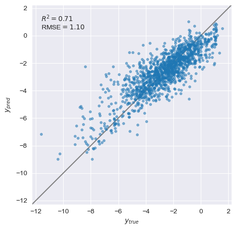
5-foldのOut-of-fold予測値を算出する。
estimator = RandomForestRegressor(random_state=334, n_jobs=-1)
y_oof = cross_val_predict(
    estimator,
    X_selected,
    y,
    cv=KFold(n_splits=5, shuffle=True, random_state=SEED),
    n_jobs=-1,
)
# true vs pred
def yyplot(
    y: Union[pd.Series, np.ndarray], y_pred: Union[pd.Series, np.ndarray]
) -> None:

    sns.set_style("darkgrid")

    fig, ax = plt.subplots(facecolor="w")

    _tmp = np.hstack([np.array(y).ravel(), np.array(y_pred).ravel()])
    _range = (min(_tmp), max(_tmp))
    alpha = 0.05
    offset = (max(_range) - min(_range)) * alpha
    _plot_range = (min(_tmp) - offset, max(_tmp) + offset)

    ax.plot(*[_plot_range] * 2, color="gray", zorder=1)
    ax.scatter(y, y_pred, marker="o", s=10, alpha=0.5)

    ax.set_xlabel("$y_{true}$")
    ax.set_ylabel("$y_{pred}$")

    ax.set_xlim(_plot_range)
    ax.set_ylim(_plot_range)

    ax.text(
        min(_range),
        max(_range),
        f"$R^2={r2_score(y, y_pred):.2g}$\nRMSE$={mean_squared_error(y, y_pred, squared=False):.2f}$",
        ha="left",
        va="top",
    )

    ax.set_aspect("equal")
    fig.tight_layout()
yyplot(y, y_oof)
ホールドアウト法による学習モデルの構築
X_train_selected, X_test_selected, y_train, y_test = train_test_split(
    X_selected, y, test_size=0.2, random_state=SEED
)
estimator.fit(X_train_selected, y_train)

y_pred_on_train = estimator.predict(X_train_selected)
y_pred_on_test = estimator.predict(X_test_selected)
# true vs pred
def yyplot_train_test(
    y_train: Union[pd.Series, np.ndarray],
    y_pred_on_train: Union[pd.Series, np.ndarray],
    y_test: Union[pd.Series, np.ndarray],
    y_pred_on_test: Union[pd.Series, np.ndarray],
) -> None:

    sns.set_style("darkgrid")

    fig, ax = plt.subplots(facecolor="w")

    _tmp = np.hstack(
        [
            np.array(_y).ravel()
            for _y in [y_train, y_pred_on_train, y_test, y_pred_on_test]
        ]
    )
    _range = (min(_tmp), max(_tmp))
    alpha = 0.05
    offset = (max(_range) - min(_range)) * alpha
    _plot_range = (min(_tmp) - offset, max(_tmp) + offset)

    ax.plot(*[_plot_range] * 2, color="gray", zorder=1)
    ax.scatter(
        y_train, y_pred_on_train, marker="o", s=10, alpha=0.5, label="train"
    )
    ax.scatter(
        y_test, y_pred_on_test, marker="o", s=10, alpha=0.5, label="test"
    )

    ax.set_xlabel("$y_{true}$")
    ax.set_ylabel("$y_{pred}$")

    ax.set_xlim(_plot_range)
    ax.set_ylim(_plot_range)

    ax.text(
        min(_range),
        max(_range),
        "train\n"
        + f"$R^2={r2_score(y_train, y_pred_on_train):.2g}$\n"
        + f"RMSE$={mean_squared_error(y_train, y_pred_on_train, squared=False):.2f}$\n"
        "\ntest\n"
        + f"$R^2={r2_score(y_test, y_pred_on_test):.2g}$\n"
        + f"RMSE$={mean_squared_error(y_test, y_pred_on_test, squared=False):.2f}$",
        ha="left",
        va="top",
    )

    ax.set_aspect("equal")
    fig.tight_layout()
yyplot_train_test(y_train, y_pred_on_train, y_test, y_pred_on_test)
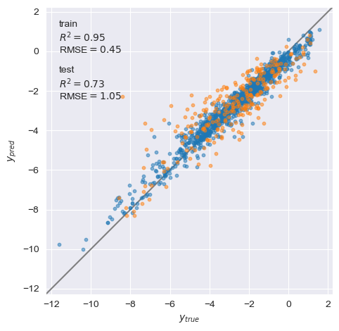
少し過学習気味なので、ハイパーパラメータのチューニングなどが必要かもしれない。
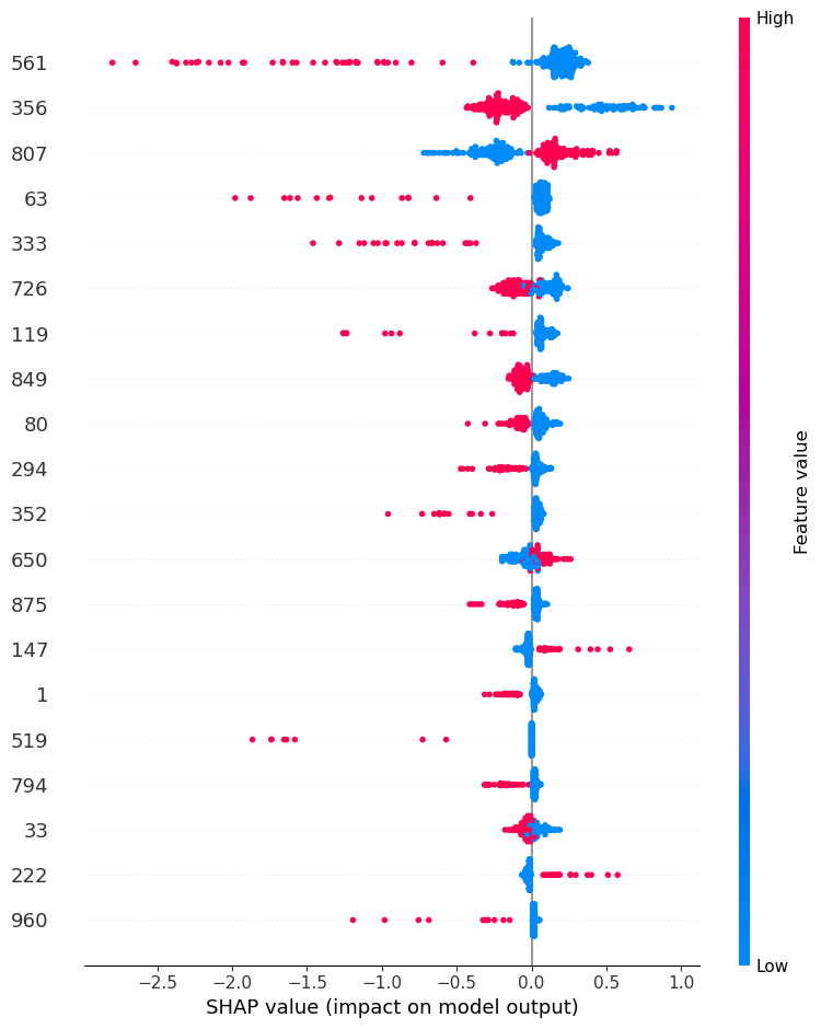
SHAP値の算出
explainer = shap.TreeExplainer(estimator, X_test_selected)
shap_values = pd.DataFrame(
    explainer.shap_values(X_test_selected),
    index=X_test_selected.index,
    columns=X_test_selected.columns,
)
plt.rcParams.update(plt.rcParamsDefault)
shap.summary_plot(shap_values.values, X_test_selected, plot_type="dot")
shap_values.shape
(258, 185)
部分構造の寄与の可視化
部分構造の寄与は以下の式で計算される。
\[A_i = \sum_{n=1}^{N} \left( C_n \times \frac{1}{f_n} \times \frac{1}{x_n} \right)\]- $C_n$: 各フィンガープリントの寄与
- $f_n$: 分子中に含まれる各部分構造の数 ($n = 1, 2, \ldots, N$)
- $x_n$: 各部分構造に含まれる原子数
これを関数化した。
def visualize_importance_atoms(
    mol: Chem.rdchem.Mol,
    bitinfo: Dict[int, Tuple[Tuple[int, int]]],
    ratio_contribution: Union[Dict[int, float], pd.Series],
    legend: Optional[str] = None,
    save_as: Optional[Literal["*.svg"]] = None,
) -> str:
    """visualize importance atoms

    Parameters
    ----------
    mol : Chem.rdchem.Mol
        rdkit mol object
    bitinfo : Dict[int, Tuple[Tuple[int, int]]]
        bitinfo, key is bit number, value is tuple of (atom index, radius)
    ratio_contribution : Union[Dict[int, float], pd.Series]
        contribution of each bit, key is bit number, value is contribution
    legend : Optional[str], optional
        legend, by default None
    save_as : Optional[Literal[*.svg]], optional
        save filepath of svg, by default None

    Returns
    -------
    str
        svg string
    """

    if type(ratio_contribution) == pd.Series:
        ratio_contribution = ratio_contribution.to_dict()

    bit_list = list(set(bitinfo.keys()) & set(ratio_contribution.keys()))

    importance_atoms = np.zeros(mol.GetNumAtoms(), dtype=float)
    for _bit in bit_list:
        n_substructure = len(bitinfo[_bit])
        contribution: float = ratio_contribution[_bit]
        for i_atom, radius in bitinfo[_bit]:
            if radius == 0:
                n_atom_in_substructure = 1
                importance_atoms[i_atom] += (
                    contribution / n_atom_in_substructure / n_substructure
                )
            else:
                atom_map = {}
                env = Chem.FindAtomEnvironmentOfRadiusN(
                    mol, radius=radius, rootedAtAtom=i_atom
                )
                submol = Chem.PathToSubmol(mol, env, atomMap=atom_map)

                n_atom_in_substructure = len(submol.GetAtoms())
                for j_atom in atom_map:
                    importance_atoms[j_atom] += (
                        contribution / n_atom_in_substructure
                    )

    # scaling
    importance_atoms_scaled = (
        importance_atoms / abs(importance_atoms).max() * 0.5
    )

    atom_colors: Dict[int, Tuple[float, float, float]] = {
        i: (
            1.0,
            1 - importance_atoms_scaled[i],
            1 - importance_atoms_scaled[i],
        )
        if importance_atoms_scaled[i] > 0
        else (
            1 + importance_atoms_scaled[i],
            1 + importance_atoms_scaled[i],
            1.0,
        )
        for i in range(len(importance_atoms_scaled))
    }

    view = Draw.rdMolDraw2D.MolDraw2DSVG(300, 300)
    tm = Draw.rdMolDraw2D.PrepareMolForDrawing(mol)
    view.DrawMolecule(
        tm,
        highlightAtoms=atom_colors.keys(),
        highlightAtomColors=atom_colors,
        highlightBonds=[],
        highlightBondColors={},
        legend=legend,
    )
    view.FinishDrawing()
    svg = view.GetDrawingText()

    if save_as is not None and os.path.basename(save_as).endswith(".svg"):
        with open(save_as, mode="w", encoding="utf-8") as f:
            f.write(svg)
    return svg
予測値と実際の値が近いトップ3の分子を可視化
indices = (
    (y_test - y_pred_on_test)
    .abs()
    .reset_index()
    .sort_values(by=target_col)
    .index.tolist()[:3]
)
for i in indices:
    bitinfo = bitinfos[i]
    ratio_contribution: pd.Series = shap_values.iloc[i]  # C_n
    mol = df_extracted["ROMol"][i]
    legend = f"y_true: {y_test[i]:.2f}  y_pred: {y_pred_on_test[i]:.2f}"

    svg = visualize_importance_atoms(
        mol=mol,
        ratio_contribution=ratio_contribution,
        bitinfo=bitinfo,
        legend=legend,
    )
    display(SVG(svg))


赤が目的変数に正の影響、青が目的変数に負の影響を与えることを示す。色の濃さがその影響の強さを示す。
注意点
以上で示したのは、部分構造の寄与をそれぞれの化合物ごとに示した結果である。
つまり、分子間で同じ色の濃さを示している部分であってもスケールが異なるため単純に比較できない。
これを揃えるためには、scalingの部分を共通の関数で行う必要がある。
また、後述するが、あくまで部分構造の有無から算出した値であることにも注意が必要である。
この手法の欠点
以下に個人的に考えたこの手法の欠点を挙げる。
- モデルが正しくない場合、誤った解釈をおこなってしまう可能性がある
- bitのフィンガープリントを用いているため、部分構造の “数” が無視されている
1についてはどの解釈手法でも言えることであるが、モデルを解釈する手法である以上、モデル自体が間違っていた場合、正しい結果は得られないことを頭の片隅に入れておくべきである。
2については、この手法はあくまで部分構造があるかないかを(1, 0)で示しているbitのフィンガープリントを特徴量として用いているので、部分構造が多ければ多いほど、のような解釈は与えられない。これは間違った解釈をしやすい部分であるので改善の余地があるように思う。
まとめ
以上のように可視化には成功した。
その一方で、これらの結果がドメイン知識に一致しているかというと、あまり一致していないように感じるので、やはりモデルが正しく構築できていないのだと思う。
このようにモデルの正しさを検討する材料のうちの一つになりえる。
いくつか改善の余地はあるが、正しいモデルを構築できれば、見栄えが良くかつ説得力のある説明ができる素晴らしい手法であると思う。