【Python】内挿・外挿の判定
目次
自分が使う、外れ値検出手法についてのまとめ。
説明については各サイトに譲り、使い方をサンプルデータを使って示す。
Sponsored by Google AdSense
使い分け
金子先生曰く以下。
- k近傍法
- データ分布に違いがあると対応が難しい
- 次元の呪いの影響を受ける
- OCSVM
- データ分布に違いがあると対応が難しい
- 次元の呪いの影響を受けにくい
- LOF
- データ分布に違いがあっても対応できる
- 次元の呪いの影響を受ける
参考: Local Outlier Factor (LOF)
使い方
実装
パッケージのインストール
import os
import sys
from urllib import request

import numpy as np
import pandas as pd
import sklearn
import scipy
import matplotlib as mpl
import matplotlib.pyplot as plt
from sklearn.model_selection import train_test_split
from sklearn.ensemble import RandomForestRegressor
from sklearn.metrics import mean_squared_error
print(f'Python: {sys.version}')

for package in (np, pd, sklearn, scipy, mpl):
    print(f'{package.__name__}: {package.__version__}')
Python: 3.8.13 | packaged by conda-forge | (default, Mar 25 2022, 06:05:16)
[Clang 12.0.1 ]
numpy: 1.23.1
pandas: 1.4.3
sklearn: 1.1.2
scipy: 1.9.0
matplotlib: 3.5.2
サンプルデータセットの準備
# 配布ページ: https://datachemeng.com/pythonassignment/
url = 'https://datachemeng.com/wp-content/uploads/2017/07/logSdataset1290.csv'

dirpath_cache = os.path.abspath('./_cache')
if not os.path.isdir(dirpath_cache):
    os.mkdir(dirpath_cache)

fpath_csv_cache = os.path.join(dirpath_cache, os.path.basename(url))
if not os.path.isfile(fpath_csv_cache):
    with request.urlopen(url) as response:
        content = response.read().decode('utf-8-sig')
    with open(fpath_csv_cache, 'w', encoding='utf-8-sig') as f:
        f.write(content)

df_data = pd.read_csv(fpath_csv_cache, index_col=0)
df_data.head()
| logS | MolWt | HeavyAtomMolWt | ExactMolWt | NumValenceElectrons | NumRadicalElectrons | MaxPartialCharge | MinPartialCharge | MaxAbsPartialCharge | MinAbsPartialCharge | ... | fr_sulfide | fr_sulfonamd | fr_sulfone | fr_term_acetylene | fr_tetrazole | fr_thiazole | fr_thiocyan | fr_thiophene | fr_unbrch_alkane | fr_urea | |
|---|---|---|---|---|---|---|---|---|---|---|---|---|---|---|---|---|---|---|---|---|---|
| CC(N)=O | 1.58 | 59.068 | 54.028 | 59.037114 | 24 | 0 | 0.213790 | -0.369921 | 0.369921 | 0.213790 | ... | 0 | 0 | 0 | 0 | 0 | 0 | 0 | 0 | 0 | 0 |
| CNN | 1.34 | 46.073 | 40.025 | 46.053098 | 20 | 0 | -0.001725 | -0.271722 | 0.271722 | 0.001725 | ... | 0 | 0 | 0 | 0 | 0 | 0 | 0 | 0 | 0 | 0 |
| CC(=O)O | 1.22 | 60.052 | 56.020 | 60.021129 | 24 | 0 | 0.299685 | -0.481433 | 0.481433 | 0.299685 | ... | 0 | 0 | 0 | 0 | 0 | 0 | 0 | 0 | 0 | 0 |
| C1CCNC1 | 1.15 | 71.123 | 62.051 | 71.073499 | 30 | 0 | -0.004845 | -0.316731 | 0.316731 | 0.004845 | ... | 0 | 0 | 0 | 0 | 0 | 0 | 0 | 0 | 0 | 0 |
| NC(=O)NO | 1.12 | 76.055 | 72.023 | 76.027277 | 30 | 0 | 0.335391 | -0.349891 | 0.349891 | 0.335391 | ... | 0 | 0 | 0 | 0 | 0 | 0 | 0 | 0 | 0 | 1 |
5 rows × 197 columns
col_target = 'logS'
X = df_data.drop(col_target, axis=1)
y = df_data[col_target]
X_train, X_test, y_train, y_test = train_test_split(X, y, test_size=0.2, random_state=334)
# 型付け
X_train:pd.DataFrame
X_test:pd.DataFrame
y_train:pd.Series
y_test:pd.Series
比較のために予測モデルを作っておく
rf = RandomForestRegressor(random_state=334, n_jobs=-1)
rf.fit(X_train, y_train)
y_pred_on_train = rf.predict(X_train)
y_pred_on_test = rf.predict(X_test)
k近傍法による検出
参考
実装
ライブラリのインストール
from sklearn.neighbors import NearestNeighbors
標準化。分散が0の特徴量を削除するべきかは議論の余地があるが、今回はエラーが起きないようにかつ距離が遠いものとしてプログラム上で扱えるように分散が$0$のものを$10^{-10}$として扱うことにした。
X_train_std = X_train.std(axis=0, ddof=1)
X_train_std = X_train_std + (X_train_std == 0).astype(float) * 1e-10

X_train_scaled = (X_train - X_train.mean(axis=0)) / X_train_std
X_test_scaled = (X_test - X_train.mean(axis=0)) / X_train_std

X_train_scaled.head()
| MolWt | HeavyAtomMolWt | ExactMolWt | NumValenceElectrons | NumRadicalElectrons | MaxPartialCharge | MinPartialCharge | MaxAbsPartialCharge | MinAbsPartialCharge | MaxEStateIndex | ... | fr_sulfide | fr_sulfonamd | fr_sulfone | fr_term_acetylene | fr_tetrazole | fr_thiazole | fr_thiocyan | fr_thiophene | fr_unbrch_alkane | fr_urea | |
|---|---|---|---|---|---|---|---|---|---|---|---|---|---|---|---|---|---|---|---|---|---|
| COc1ccc2c(c1OC)C(=O)OC2C1c2cc3c(cc2CCN1C)OCO3 | 1.943717 | 1.911861 | 1.951641 | 2.294076 | 0.0 | 1.217935 | -1.066686 | 1.047323 | 1.317377 | 1.255729 | ... | -0.13317 | -0.203672 | -0.062348 | -0.076435 | 0.0 | -0.053969 | 0.0 | -0.076435 | -0.230951 | -0.19898 |
| CC(=O)Oc1c(C(C)(C)C)cc([N+](=O)[O-])c(C)c1[N+](=O)[O-] | 1.020198 | 1.012031 | 1.026183 | 1.319250 | 0.0 | 1.057576 | -0.572522 | 0.547254 | 1.144343 | 0.822041 | ... | -0.13317 | -0.203672 | -0.062348 | -0.076435 | 0.0 | -0.053969 | 0.0 | -0.076435 | -0.230951 | -0.19898 |
| Cc1ccc(C)c2ccccc12 | -0.464401 | -0.479106 | -0.462517 | -0.325769 | 0.0 | -1.459468 | 1.818841 | -1.872681 | -1.326135 | -1.839169 | ... | -0.13317 | -0.203672 | -0.062348 | -0.076435 | 0.0 | -0.053969 | 0.0 | -0.076435 | -0.230951 | -0.19898 |
| c1ccc2nc3ccccc3cc2c1 | -0.220655 | -0.193878 | -0.218174 | -0.142989 | 0.0 | -0.815132 | 0.573027 | -0.611982 | -0.876381 | -1.136818 | ... | -0.13317 | -0.203672 | -0.062348 | -0.076435 | 0.0 | -0.053969 | 0.0 | -0.076435 | -0.230951 | -0.19898 |
| C=CCC1(C(C)CCC)C(=O)NC(=S)NC1=O | 0.575786 | 0.530329 | 0.579681 | 0.709984 | 0.0 | 0.464190 | 0.211073 | -0.245703 | 0.504056 | 1.075629 | ... | -0.13317 | -0.203672 | -0.062348 | -0.076435 | 0.0 | -0.053969 | 0.0 | -0.076435 | -0.230951 | -0.19898 |
5 rows × 196 columns
# p=2: Euclidean distance
nn = NearestNeighbors(n_neighbors=5, p=2, n_jobs=-1)
nn.fit(X_train_scaled)
distance_train_, _indices = nn.kneighbors(return_distance=True)

distance_train_mean_ = np.mean(distance_train_, axis=1)
distance_threshold:float = np.percentile(distance_train_mean_, 99.7)
distance_test_, _indices = nn.kneighbors(X_test_scaled, return_distance=True)
distance_test_mean_ = np.mean(distance_test_, axis=1)
flag_inlier_train_knn = distance_train_mean_ < distance_threshold
flag_inlier_test_knn = distance_test_mean_ < distance_threshold
def make_plot(flag_inlier_train, flag_inlier_test):
    plt.close()

    # style
    mpl.style.use('seaborn-darkgrid')
    fig, ax = plt.subplots(facecolor='w', dpi=144)

    # aspect
    ax.set_aspect('equal')

    # range
    _y_tmp = np.hstack([np.array(_y).ravel() for _y in (y_train, y_test, y_pred_on_train, y_pred_on_test)])
    _range = (_y_tmp.min(), _y_tmp.max())
    alpha = 0.05
    offset = (max(_range) - min(_range)) * alpha
    _plot_range = (min(_range) - offset, max(_range) + offset)

    ax.set_xlim(_plot_range)
    ax.set_ylim(_plot_range)

    # label
    ax.set_xlabel('y_true')
    ax.set_ylabel('y_pred')

    ax.plot(*[_plot_range]*2, c='gray', zorder=1)

    # train
    ax.scatter(y_train[flag_inlier_train], y_pred_on_train[flag_inlier_train], c='C1', label='train inlier')
    ax.scatter(y_train[~flag_inlier_train], y_pred_on_train[~flag_inlier_train], c='C1', alpha=0.5, label='train outlier')

    # test
    ax.scatter(y_test[flag_inlier_test], y_pred_on_test[flag_inlier_test], c='C0', label='test inlier')
    ax.scatter(y_test[~flag_inlier_test], y_pred_on_test[~flag_inlier_test], c='C0', alpha=0.5, label='test outlier')

    # legend
    ax.legend()

    fig.tight_layout()

    # scores
    rmse_test_inlier = mean_squared_error(y_test[flag_inlier_test], y_pred_on_test[flag_inlier_test], squared=False)
    rmse_test_outlier = mean_squared_error(y_test[~flag_inlier_test], y_pred_on_test[~flag_inlier_test], squared=False)
    print(f'RMSE test inlier: {rmse_test_inlier:.3f} ({np.sum(flag_inlier_test)} samples)')
    print(f'RMSE test outlier: {rmse_test_outlier:.3f} ({np.sum(~flag_inlier_test)} samples)')
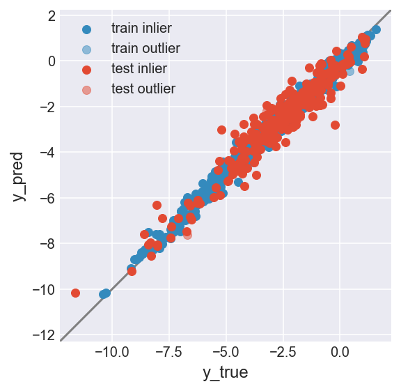
make_plot(flag_inlier_train_knn, flag_inlier_test_knn)
RMSE test inlier: 0.575 (255 samples)
RMSE test outlier: 0.821 (3 samples)
Local Outlier Factor
参考
実装
from sklearn.neighbors import LocalOutlierFactor
lof = LocalOutlierFactor(n_neighbors=5, novelty=True, contamination='auto', p=2, n_jobs=-1).fit(X_train_scaled)
flag_inlier_train_lof = lof.predict(X_train_scaled) == 1
flag_inlier_test_lof = lof.predict(X_test_scaled) == 1
/Users/yu9824/miniforge3/envs/outlier-detection/lib/python3.8/site-packages/sklearn/base.py:450: UserWarning: X does not have valid feature names, but LocalOutlierFactor was fitted with feature names
  warnings.warn(
/Users/yu9824/miniforge3/envs/outlier-detection/lib/python3.8/site-packages/sklearn/base.py:450: UserWarning: X does not have valid feature names, but LocalOutlierFactor was fitted with feature names
  warnings.warn(
make_plot(flag_inlier_train_lof, flag_inlier_test_lof)
RMSE test inlier: 0.554 (204 samples)
RMSE test outlier: 0.665 (54 samples)

One-Class Support Vector Machine
参考
実装
from sklearn.svm import OneClassSVM
ocsvm = OneClassSVM(kernel='rbf', nu=0.1, gamma='auto').fit(X_train_scaled)
flag_inlier_train_ocsvm = ocsvm.predict(X_train_scaled) == 1
flag_inlier_test_ocsvm = ocsvm.predict(X_test_scaled) == 1
make_plot(flag_inlier_train_ocsvm, flag_inlier_test_ocsvm)
RMSE test inlier: 0.561 (214 samples)
RMSE test outlier: 0.659 (44 samples)