ゼロから作るDeep Learning 第3章ニューラルネットワークを読んで取ったノートです．ご参考になれば幸いです．

本はこちら．

ゼロから作るDeep Learning

posted with ヨメレバ

斎藤康毅オライリー・ジャパン 2016年09月24日頃

楽天ブックス

Amazon

Kindle

パーセプトロンからニューラルネットワークへ

ニューラルネットワークの例

入力層・中間層（隠れ層）・出力層

引用元：https://www.sbbit.jp/article/image/33345/l_bit201703022247425548.jpg

パーセプトロンの復習

y = {\begin{cases} 0 (b + w_{1} x_{1} + w_{2} x_{2} \leq 0) \\ 1 (b + w_{1} x_{1} + w_{2} x_{2} > 0) \end{cases}

書き換えると，

\begin{array}{r} y = h (b + w_{1} x_{1} + w_{2} x_{2}) \\ h (x) = {\begin{cases} 0 (x \leq 0) \\ 1 (x > 0) \end{cases} \end{array}

活性化関数の登場

一つ目の式をより丁寧に書くと， $\begin{aligned} a & = b + w_{1} x_{1} + w_{2} x_{2} \\ y & = h (a) \end{aligned}$

$h (x)$ : 活性化関数 (activation function)
活性化関数は入力信号の総和がどのように活性化するかということを決定する．

活性化関数

単純パーセプトロンでは活性化関数にステップ関数を利用しているということができる．

シグモイド関数

h (x) = \frac{1}{1 + \exp (- x)}

ステップ関数の実装

In [1]:

                              def step_function(x):
    return int(x > 0)

np.ndarrayを入力できるように書き換え

In [2]:

                              def step_function(x):
    return (x > 0).astype(np.int64)

ステップ関数のグラフ

In [3]:

                              import numpy as np
import matplotlib.pyplot as plt

plt.rcParams['font.size'] = 13
plt.rcParams['font.family'] = 'Helvetica'

x = np.arange(-5.0, 5.0, 0.1)
y = step_function(x)

fig, ax = plt.subplots(dpi=100, facecolor='white')
ax.plot(x, y)

ax.set_xlabel('$x$')
ax.set_ylabel('$y$')

ax.set_ylim(-0.1, 1.1)

fig.tight_layout()

                         

シグモイド関数の実装

In [4]:

                              def sigmoid(x):
    return 1 / (1 + np.exp(-x))

In [5]:

                              x = np.array([-1.0, 1.0, 2.0])
sigmoid(x)

Out[5]:

array([0.26894142, 0.73105858, 0.88079708])

In [6]:

                              plt.close()

x = np.arange(-5.0, 5.0, 0.1)
y = sigmoid(x)

fig, ax = plt.subplots(dpi=100, facecolor='white')
ax.plot(x, y)

ax.set_xlabel('$x$')
ax.set_ylabel('$y$')

ax.set_ylim(-0.1, 1.1)

fig.tight_layout()

シグモイド関数とステップ関数の比較

シグモイド関数の特徴
- 滑らかで，連続値を取れる．
- 0, 1以外の値を取れる．
共通点
- 大きいと1に(近く)なるし，小さいと0に(近く)なる．
- どんな実数が入力されても0から1の間に押し込める．

非線形関数

上記以外の共通点：いずれも非線形関数であること

ニューラルネットワークでは線形関数は用いることができないため，とても重要．

線形関数の問題点は，どんなに層を深くしても，それと同じことを行う「隠れ層のないネットワーク」が必ず存在する，

（感覚的に理解できる説明だと $h (x) = c x$ とすると， $h (h (h (x))) = c^{3} x = a x (a = c^{3})$ と隠れ層なしのネットワークで表現できてしまうため）

ReLU関数

Rectified Linear Unit $h (x) = {\begin{cases} x (x > 0) \\ 0 (x \leq 0) \end{cases}$

In [7]:

                              def relu(x):
    return np.maximum(0, x)

多次元配列の計算

多次元配列

In [8]:

                              A = np.array([1, 2, 3, 4])
A

Out[8]:

array([1, 2, 3, 4])

In [9]:

np.ndim(A)

Out[9]:

In [10]:

A.shape

Out[10]:

(4,)

In [11]:

A.shape[0]

Out[11]:

In [12]:

                              B = np.array([[1, 2], [3, 4], [5, 6]])
B

Out[12]:

array([[1, 2],
       [3, 4],
       [5, 6]])

In [13]:

np.ndim(B)

Out[13]:

In [14]:

B.shape

Out[14]:

(3, 2)

行列の積

(\begin{array}{cc} 1 & 2 \\ 3 & 4 \end{array}) (\begin{array}{cc} 5 & 6 \\ 7 & 8 \end{array}) = (\begin{array}{cc} 19 & 22 \\ 43 & 50 \end{array})

In [15]:

                              A = np.array([[1, 2], [3, 4]])
B = np.array([[5, 6], [7, 8]])
np.dot(A, B)

                         

Out[15]:

array([[19, 22],
       [43, 50]])

In [16]:

                              A = np.array([[1, 2, 3], [4, 5, 6]])
B = np.array([[1, 2], [3, 4], [5, 6]])
A.shape, B.shape

                         

Out[16]:

((2, 3), (3, 2))

In [17]:

np.dot(A, B)

Out[17]:

array([[22, 28],
       [49, 64]])

In [18]:

                              C = np.array([[1, 2], [3, 4]])
A.shape, C.shape

Out[18]:

((2, 3), (2, 2))

In [19]:

                              try:
    np.dot(A, C)
except ValueError as e:
    print('{0}\nとエラーメッセージが表示される．'.format(e))

                         

shapes (2,3) and (2,2) not aligned: 3 (dim 1) != 2 (dim 0)
とエラーメッセージが表示される．

In [20]:

                              A = np.array([[1, 2], [3, 4], [5, 6]])
B = np.array([7, 8])
A.shape, B.shape

                         

Out[20]:

((3, 2), (2,))

In [21]:

np.dot(A, B)

Out[21]:

array([23, 53, 83])

ニューラルネットワークの行列の積

簡単のためにバイアスと活性化関数は省略して重みだけがあるニューラルネットワークを考える．

In [22]:

                              X = np.array([1, 2])
W = np.array([[1, 3, 5], [2, 4, 6]])
W, X.shape, W.shape

                         

Out[22]:

(array([[1, 3, 5],
        [2, 4, 6]]),
 (2,),
 (2, 3))

In [23]:

np.dot(X, W)

Out[23]:

array([ 5, 11, 17])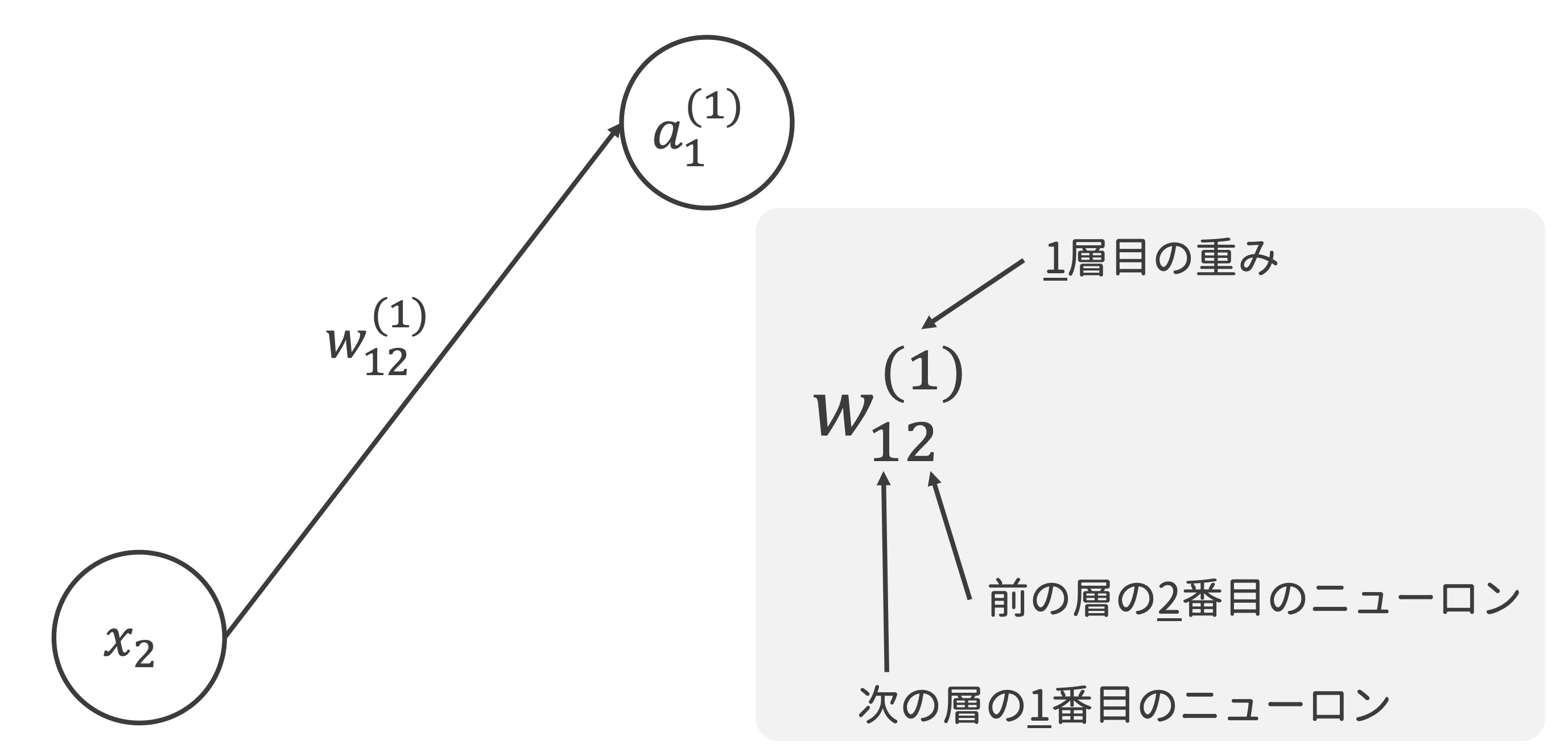

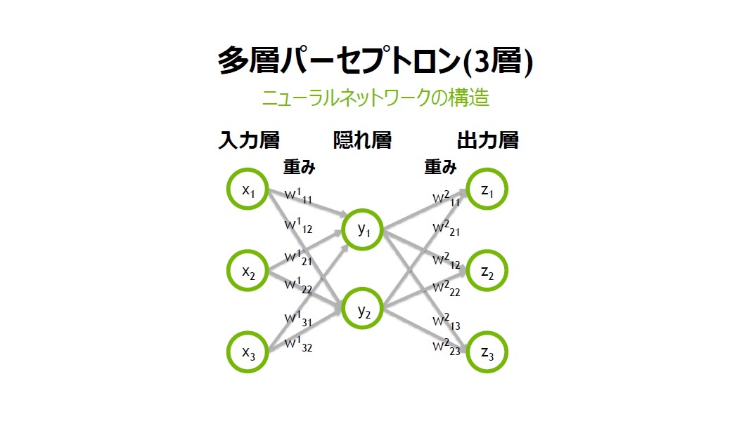
3層ニューラルネットワークの実装

記号の確認

ニューラルネットワークの一部を切り取った次の図で説明．

a_{1}^{(1)} = w_{11}^{(1)} x_{1} + w_{12} x_{2} + b_{1}^{(1)} a_{2}^{(1)} = w_{21}^{(1)} x_{1} + w_{22} x_{2} + b_{2}^{(1)} . . . a_{i}^{(1)} = w_{i 1}^{(1)} x_{1} + w_{i 2} x_{2} + b_{i}^{(1)}

これを行列で表すと $A^{(1)} = X W^{(1)} + B^{(1)}$ ただし， $A = (\begin{array}{ccc} a_{1}^{(1)} a_{2}^{(1)} a_{3}^{(1)} \end{array}) X = (\begin{array}{ccc} x_{1} x_{2} \end{array}) B = (\begin{array}{ccc} b_{1}^{(1)} b_{2}^{(1)} b_{3}^{(1)} \end{array}) W = (\begin{array}{ccc} w_{11}^{(1)} w_{21}^{(1)} w_{31}^{(1)} \\ w_{12}^{(1)} w_{22}^{(1)} w_{32}^{(1)} \end{array})$

これらをNumpyで実装．

入力層から第1層

In [24]:

                              X = np.array([1.0, 0.5])
W1 = np.array([[0.1, 0.3, 0.5], [0.2, 0.4, 0.6]])
B1 = np.array([0.1, 0.2, 0.3])

X.shape, W1.shape, B1.shape

Out[24]:

((2,), (2, 3), (3,))

In [25]:

                              A1 = np.dot(X, W1) + B1
A1

Out[25]:

array([0.3, 0.7, 1.1])

In [26]:

                              Z1 = sigmoid(A1)
Z1

Out[26]:

array([0.57444252, 0.66818777, 0.75026011])

第1層から第2層

In [27]:

                              W2 = np.array([[0.1, 0.4], [0.2, 0.5], [0.3, 0.6]])
B2 = np.array([0.1, 0.2])
Z1.shape, W2.shape, B2.shape

                         

Out[27]:

((3,), (3, 2), (2,))

In [28]:

                              A2 = np.dot(Z1, W2) + B2
Z2 = sigmoid(A2)

第2層から出力層

In [29]:

                              def identity_function(x):
    return x

W3 = np.array([[0.1, 0.3], [0.2, 0.4]])
B3 = np.array([0.1, 0.2])

A3 = np.dot(Z2, W3) + B3
Y = identity_function(A3)
Y

                         

Out[29]:

array([0.31682708, 0.69627909])

ここでのidentity_functionは恒等関数．

出力層への伝達で使われる活性化関数は， $σ (x)$ として表され，他の活性化関数とは区別して扱われる．

実装のまとめ

In [30]:

                              def init_network():
    network = dict(
        W1 = np.array([[0.1, 0.3, 0.5], [0.2, 0.4, 0.6]]),
        b1 = np.array([0.1, 0.2, 0.3]),
        W2 = np.array([[0.1, 0.4], [0.2, 0.5], [0.3, 0.6]]),
        b2 = np.array([0.1, 0.2]),
        W3 = np.array([[0.1, 0.3], [0.2, 0.4]]),
        b3 = np.array([0.1, 0.2]),
    )
    return network

                         

In [31]:

                              def forward(network, x):
    W1, W2, W3 = network['W1'], network['W2'], network['W3']
    b1, b2, b3 = network['b1'], network['b2'], network['b3']

    # 入力層から第1層
    a1 = np.dot(x, W1) + b1
    z1 = sigmoid(a1)
    # 第1層から第2層
    a2 = np.dot(z1, W2) + b2
    z2 = sigmoid(a2)
    # 第2層から出力層
    a3 = np.dot(z2, W3) + b3
    y = identity_function(a3)
    return y

                         

In [32]:

                              network = init_network()
x = np.array([1.0, 0.5])
y = forward(network, x)
y

                         

Out[32]:

array([0.31682708, 0.69627909])

出力層の設計

出力層の活性化関数を変更することで分類問題，回帰問題どちらにも用いることができる．一般に，

回帰問題: 恒等関数
分類問題: ソフトマックス関数

恒等関数とソフトマックス関数

恒等関数 $y_{k} = a_{k}$

ソフトマックス関数 $y_{k} = \frac{\exp a_{k}}{\sum_{i = 1}^{n} \exp a_{i}}$

→ 出力の各ニューロンがすべての入力信号から影響を受ける．

ソフトマックス関数を実装．

In [33]:

                              a = np.array([0.3, 2.9, 4.0])

exp_a = np.exp(a)
exp_a

Out[33]:

array([ 1.34985881, 18.17414537, 54.59815003])

In [34]:

                              sum_exp_a = np.sum(exp_a)
sum_exp_a

Out[34]:

74.1221542101633

In [35]:

                              y = exp_a / sum_exp_a
y

Out[35]:

array([0.01821127, 0.24519181, 0.73659691])

関数化すると，

In [36]:

                              def softmax(a):
    exp_a = np.exp(a)
    sum_exp_a = np.sum(exp_a)
    y = exp_a / sum_exp_a
    return y

                         

ソフトマックス関数の実装上の注意

オーバーフロー問題：指数関数は容易に膨大な桁数になってしまう可能性があり，数値が「不安定」になってしまう．

これを解決するため以下の式変形を行う． $\begin{aligned} y_{k} & = \frac{\exp a_{k}}{\sum_{i = 1}^{n} \exp a_{i}} \\ = \frac{C^{'} \exp a_{k}}{C^{'} \sum_{i = 1}^{n} \exp a_{i}} \\ = \frac{\exp (a_{k} + \log C^{'})}{\sum_{i = 1}^{n} \exp (a_{i} + \log C^{'})} \\ = \frac{\exp (a_{k} + C)}{\sum_{i = 1}^{n} \exp (a_{i} + C)} (C = \log C^{'}) \end{aligned}$ このとき， $C^{'}, C$ は任意の定数．

オーバーフローしてしまう例

In [37]:

                              a = np.array([1010, 1000, 990])
np.exp(a) / np.sum(np.exp(a))

<ipython-input-37-23103c906500>:2: RuntimeWarning: overflow encountered in exp
  np.exp(a) / np.sum(np.exp(a))
<ipython-input-37-23103c906500>:2: RuntimeWarning: invalid value encountered in true_divide
  np.exp(a) / np.sum(np.exp(a))

Out[37]:

array([nan, nan, nan])

そこで先程の式変形の要領で改善してみる．

In [38]:

                              c = np.max(a)
a - c

Out[38]:

array([  0, -10, -20])

In [39]:

np.exp(a - c) / np.sum(np.exp(a - c))

Out[39]:

array([9.99954600e-01, 4.53978686e-05, 2.06106005e-09])

In [40]:

                              def softmax(a):
    c = np.max(a)
    exp_a = np.exp(a - c)   # オーバーフロー対策
    sum_exp_a = np.sum(exp_a)
    y = exp_a / sum_exp_a
    return y

                         

ソフトマックス関数の特徴

出力の総和が1になる．→ 確率として解釈できる．

In [41]:

                              a = np.array([0.3, 2.9, 4.0])
y = softmax(a)
y

                         

Out[41]:

array([0.01821127, 0.24519181, 0.73659691])

In [42]:

np.sum(y)

Out[42]:

1.0

y[0]: 1.8 %の確率
y[1]: 24.5 %の確率
y[2]: 73.7 %の確率

と解釈することができ，確率的（統計的）な対応が可能！

注意点

ソフトマックス関数を適用しても大小関係は変わらない．
- 指数関数が単調増加関数であることに起因
- 実際の問題で分類を行う際ソフトマックス関数は省略されることが一般的．

出力層のニューロンの数

分類したいクラスの数に設定するのが一般的．

手書き数字認識

実践的な問題にチャレンジ．

推論処理のみを実装．

MNISTデータセット

MNIST: 手書き数字の画像セット．

訓練画像: 60,000枚
テスト画像: 10,000枚

今回は配布プログラムをインポートして，データを取得．

In [43]:

                              import sys, os
sys.path.insert(0, os.path.dirname(os.path.abspath('')))    # 上の階層のモジュールをインポートすることができないので．

In [44]:

from dataset.mnist import load_mnist

In [45]:

                              (X_train, t_train), (X_test, t_test) = load_mnist(flatten=True, normalize=False)

                         

In [46]:

                              from PIL import Image

def img_show(img):
    # numpy.ndarray to PIL用データオブジェクト
    pil_img = Image.fromarray(np.uint8(img))
    return pil_img  # jupyter notebookなので書き換えた．

(x_train, t_train), (x_test, t_test) = load_mnist(flatten=True, normalize=False)

img = x_train[0]
label = t_train[0]
label

                         

Out[46]:

In [47]:

img.shape

Out[47]:

(784,)

In [48]:

                              # 一辺の大きさ
a = int('{0:.0f}'.format(np.sqrt(img.shape[0])))

img = img.reshape(a, a)
img.shape

Out[48]:

(28, 28)

In [49]:

img_show(img)

Out[49]:

ニューラルネットワークの推論処理

入力層: 784個 (28×28の画像)
出力層: 10個 (10個の数字ラベル)
隠れ層: 任意に設定可能．
- ひとつめ: 50個
- ふたつめ: 100個

のニューロンで構成されるニューラルネットワークを実装．

In [50]:

                              import pickle

def get_data():
    (x_train, t_train), (x_test, t_test) = load_mnist(normalize=True, flatten=True, one_hot_label=False)
    return x_test, t_test

def init_network():
    with open('sample_weight.pkl', 'rb') as f:
        network = pickle.load(f)
    return network

def predict(network, x):
    W1, W2, W3 = network['W1'], network['W2'], network['W3']
    b1, b2, b3 = network['b1'], network['b2'], network['b3']

    a1 = np.dot(x, W1) + b1
    z1 = sigmoid(a1)

    a2 = np.dot(z1, W2) + b2
    z2 = sigmoid(a2)

    a3 = np.dot(z2, W3) + b3
    y = softmax(a3)

    return y

                         

In [51]:

                              from tqdm.notebook import tqdm

x, t = get_data()
network = init_network()

accuracy_cnt = 0
for i in tqdm(range(len(x))):
    y = predict(network, x[i])
    p = np.argmax(y)
    if p == t[i]:
        accuracy_cnt += 1
print('Accuracy: {0:.4f}'.format(accuracy_cnt/len(x)))

                         

Accuracy: 0.9352

正規化 (normalization) という前処理 (pre-processing) を行っている．

バッチ処理

In [52]:

                              x, _ = get_data()
network = init_network()

W1, W2, W3 = network['W1'], network['W2'], network['W3']

x.shape

Out[52]:

(10000, 784)

In [53]:

x[0].shape

Out[53]:

(784,)

In [54]:

W1.shape, W2.shape, W3.shape

Out[54]:

((784, 50), (50, 100), (100, 10))

さっきの実装は一枚ずつ予測していた．→ バッチ処理したい！

バッチ処理: まとめて計算する．
- 一枚あたりの処理時間を減らせる．

In [55]:

                              x, t = get_data()
network = init_network()

batch_size = 100    # バッチの数
accuracy_cnt = 0

for i in tqdm(range(0, len(x), batch_size)):
    x_batch = x[i:i+batch_size]
    y_batch = predict(network, x_batch)
    p = np.argmax(y_batch, axis=1)
    accuracy_cnt += np.sum(p == t[i:i+batch_size])
print('Accuracy: {:.4f}'.format(accuracy_cnt / len(x)))

                         

Accuracy: 0.9352

まとめ

ニューラルネットワークでは，活性化関数としてシグモイド関数やReLU関数のような滑らかに変化する関数を利用する．

NumPyの多次元配列をうまく使うことで，ニューラルネットワークを効率よく実装することができる．

機械学習の問題は，回帰問題と分類問題に大別できる．

出力層で使用する活性化関数は，回帰問題では恒等関数，分類問題ではソフトマックス関数を一般的に利用する．

分類問題では，出力層のニューロンの数を分類するクラス数に設定する．

入力データのまとまりをバッチといい，バッチ単位で推論処理を行うことで，計算を高速に行うことができる．